Land Cover Clustering in the Upper Santa Maria Creek Subwatershed, California
Using multispectral satellite imagery and unsupervised classification to interpret vegetation, bare ground, and built environments around Ramona, CA
In this project, I use multispectral satellite imagery to explore land-cover variation in the Upper Santa Maria Creek subwatershed (HUC12 180703040203), an inland headwater subwatershed that overlaps north-central Ramona, California. This landscape is a useful case for unsupervised classification because it includes a developed town center, dry grasslands and shrublands, oak-lined ravines, bare soil, and surrounding uplands within a relatively compact watershed.
Rather than starting with pre-labeled land-cover classes, I use KMeans clustering to group pixels by their spectral similarity. The goal is not to produce a final land-cover map, but to ask whether the satellite data can reveal meaningful spatial patterns in a dry, heterogeneous Southern California watershed.
You can find the notebook code here.
Why this watershed?
The Upper Santa Maria Creek Sub-watershed (HUC12 180703040203) is an inland headwater sub-watershed in California, (technically) within San Diego County, and is part of the larger San Dieguito River watershed system that runs from the eastern mountain range all the way to the ocean (see figure 1). I say that the Santa Maria Creek Sub-watershed is “technically” within San Diego County, because the town that occupies all the wastershed boundaries is an unincorporated community of San Diego county.
This area is typically dry and we are often subject to flashflooding due to compaction and drought conditions. So often the watershed doesn’t appear to be much of a watershed. If you check out the USGS station for this location (11028500), we have very little stream flow and occasional larger storm events (like the winter of 2026).
This sub-watershed lies in north-central Ramona, CA and adjacent uplands, draining generally northwesterly toward the San Pasqual Valley area where Santa Maria Creek meets Santa Ysabel Creek to form the San Dieguito River.
As one might expect, this subwatershed like many others in California is under climate stress. Ramona relies on water pumped up from the lower city of Poway, CA (about 1,000 feet in elevation difference). We have one main resevoir (Lake Ramona), but in general all of our other water is from groundwater. This particular sub-watershed is typically very dry and much of its recharge capabilities has been negatively impacted by the construction of the town in the sub-watershed basin area.
Personally, I think the feature of this subwatershed is interesting to explore from both an ecological and land-use perspective as it is a place where vegetation, built infrastructure, water, and climate stress are tightly connected.
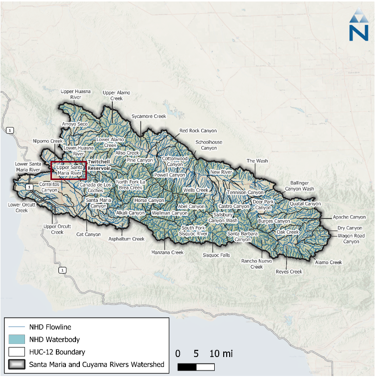
Figure 1: Santa Maria and Cuyama Rivers watershed with the Upper Santa Maria Subwatershed in red (original figure from Paradigm Environmental, 2025).
Figure 2: Interactable map of only the Santa Maria Creek Subwatershed (HUC12 180703040203).
Project question
Since we are playing with KMeans, the central question for this project is:
How well can an unsupervised clustering workflow distinguish vegetation, bare ground, built environments, and transitional land-cover patterns in a dry Southern California subwatershed?
Because KMeans does not know what “vegetation,” “bare soil,” or “urban land” are ahead of time, the interpretation has to come from the spectral patterns, the RGB imagery, and local knowledge of the landscape.
Data and tools
For this project, I used:
- Watershed boundary: Upper Santa Maria Creek, HUC12 180703040203
- Satellite imagery: NASA Earthdata imagery accessed with
earthaccess - Spectral bands: visible, near-infrared, shortwave infrared, and thermal bands
- Clustering method: KMeans clustering with six clusters
- Primary Python tools:
geopandas,rasterio,rioxarray,xarray,earthaccess,scikit-learn,hvplot,holoviews,numpy, andpandas
Workflow
Briefly, to do the KMeans, my workflow followed five main steps:
First, I defined the study area using the HUC12 watershed boundary. This boundary set the spatial extent for the analysis and was used to clip the satellite imagery (see figure 2 above).
Second, I searched for satellite granules that intersected the watershed. Because satellite imagery is stored in tiles, a single watershed may overlap multiple granules. I pulled the relevant granules, collected metadata, and prepared the file links for each spectral band.
Third, I opened, cropped, masked, and scaled the imagery. This included clipping each band to the watershed, applying the Fmask layer to remove clouds or low-quality pixels, and checking the resulting arrays for missing values or unexpected reflectance ranges.
Fourth, I merged the image granules into a continuous multispectral composite. This produced a raster where each pixel had a vector of reflectance values across multiple wavelengths.
Finally, I reshaped the raster into a tabular format for KMeans clustering. Each row represented a pixel, and each column represented a spectral band. After removing missing or zero-value pixels, I fit the clustering model and converted the cluster labels back into a spatial map.
Why KMeans?
KMeans clustering is useful for an exploratory project because it groups pixels based on spectral similarity without requiring training data. This makes it a good first step when the goal is to understand broad landscape patterns before doing more formal classification or ground-truthing. However, it should be recognized that KMeans is more useful in cases where high quality NDVI, land cover, and other forms of spatial data is not available. In other words, for most U.S. and global north countries, KMeans can be easily substituted with more specific models and data. This process may be more useful in the global south where there is less high quality data.
For the final KMeans, I tested different cluster counts and used six clusters for the final interpretation. Six clusters provided enough detail to separate vegetation, bare soil, built environments, and mixed areas without producing a map that was too fragmented to interpret.
It is important to note that cluster labels are not physical measurements. The bands represent measured reflectance values across different wavelengths, but the cluster numbers are algorithm-generated labels. If the number of clusters changes, the labels and groupings can also change.
What the clusters show
Figure 3: This is a comparison between the satillite bands and KMeans clustering.
The final KMeans map suggests a somewhat clear gradient across the watershed, from more vegetated upland areas to drier or more developed areas in the basin.
| Cluster pattern | Land cover grouping | Interpretation details |
|---|---|---|
| Cluster 0 and 1 (dark blue and orange) | Likely vegetation | Higher near-infrared reflectance and lower red reflectance, especially in uplands and oak-lined ravines |
| Cluster 2 (green) | Moderate vegetation or mixed cover | Similar to the more vegetated cluster, but less dense or more mixed |
| Cluster 3 (lite blue) | Built environments | Bright tan and white areas in the RGB image align with much of central Ramona |
| Cluster 4 and 5 (pink and black) | Transitional built areas or bare ground | Higher shortwave infrared and red reflectance, often associated with dry or exposed surfaces |
The upland and mountainside areas are generally captured by the more vegetated clusters. Some small water features are difficult to distinguish because they occur in deep ravines with dense trees along the banks, making them spectrally similar to shaded or dense vegetation rather than open water.
The central portion of the watershed is much more strongly associated with built environments and dry exposed surfaces. This corresponds with the footprint of Ramona, which appears as brighter white and tan areas in the RGB imagery. The KMeans results captures this developed area through clusters that overlap with bare ground, roofs, roads, and other reflective urban surfaces.
Key findings
Taken together, the six clusters show that the Upper Santa Maria Creek subwatershed is not easily divided into simple land-cover categories. Instead, it is best understood as a continuum from denser vegetation in upland and ravine areas to sparse vegetation, bare soil, and built environments in the central basin.
From the KMeans, the strongest patterns were:
- A vegetation gradient from upland and mountainside areas to drier, more exposed surfaces
- A distinction between wetter or more vegetated areas and drier, more developed areas
- Clear alignment between the RGB image and the built footprint of Ramona
- Transitional zones that reflect the mixed and heterogeneous nature of the watershed
Limitations
The main limitation of this project is that KMeans is an unsupervised method. The model groups pixels by spectral similarity, but it does not know the real-world land-cover class of each pixel. This means the final interpretation is inferential and should be validated with additional data, such as field observations, land-cover reference maps, or higher-resolution imagery.
The results are also sensitive to the number of clusters selected. A five-cluster model would simplify the landscape, while a seven-cluster model might capture more local variation but be harder to interpret. Because the watershed is heterogeneous, especially where built environments meet grasslands, shrubs, and oaks, some clusters inevitably represent mixed or transitional conditions.
Seasonality is another limitation and highly relevant to understanding this subwatershed in Ramona, CA as it is a chapparal region. Summer imagery is useful for detecting dry soil, vegetation stress, and thermal differences, but it may not represent the watershed during greener months or immediately after rainfall.
Larger interpretation
Overall, KMeans clustering provides a meaningful first look at land-cover variability in the Upper Santa Maria Creek subwatershed. As mentioned earlier, the approach is especially useful for identifying where vegetation, bare soil, built environments, and mixed surfaces form visible spatial patterns.
For landscapes where high-quality land-cover data already exist, KMeans may be most useful as an exploratory or teaching tool. However, in places where land-cover reference data are limited, unsupervised clustering can provide a starting point for understanding landscape structure before ground-truthing or more advanced classification.
For this watershed, the results highlight how development, dryland vegetation, and watershed processes are intertwined. The central built environment is clearly visible in the clustering results, while the uplands and ravines retain stronger vegetation signatures. While I don’t find KMeans the best method for land-cover interpretation within U.S. contexts, I think it is a fun exercise to explore the relationships between built and natural environments using remote sensing.
Data sources
- California Nature / CDFW HUC12 watershed boundaries: Upper Santa Maria Creek, HUC12 180703040203
- NASA Earthdata satellite imagery accessed through
earthaccess - USGS streamflow context for Santa Maria Creek station 11028500
Works cited
Paradigm Environmental (2025). Work Plan: Santa Maria and Cuyama Rivers Watershed Hydrology Model Development. Accessed from: https://www.waterboards.ca.gov/waterrights/water_issues/programs/supply-and-demand/docs/santa-maria-work-plan.pdf